Interactive online version:

Using EMLP in PyTorch

So maybe you haven’t yet realized that Jax is the best way of doing deep learning – that’s ok!

You can use EMLP and the equivariant linear layers in PyTorch. Simply replace import emlp.nn as nn with import emlp.nn.pytorch as nn.

If you’re using a GPU (which we recommend), you will want to set the environment variable so that Jax doesn’t steal all of the GPU memory from PyTorch. Note that if a GPU is visible under CUDA_VISIBLE_DEVICES, you must use the PyTorch EMLP on the GPU.

%env XLA_PYTHON_CLIENT_PREALLOCATE=false

env: XLA_PYTHON_CLIENT_PREALLOCATE=false

import torch
import emlp.nn.pytorch as nn

from emlp.reps import T,V
from emlp.groups import SO13

repin= 4*V # Setup some example data representations
repout = V**0
G = SO13() # The lorentz group

device = torch.device('cuda' if torch.cuda.is_available() else 'cpu')

x = torch.randn(5,repin(G).size()).to(device) # generate some random data

model = nn.EMLP(repin,repout,G).to(device) # initialize the model

model(x)

tensor([[-0.0039],
        [-0.0041],
        [-0.0042],
        [-0.0040],
        [-0.0039]], device='cuda:0', grad_fn=<AddmmBackward>)

The model is a standard pytorch module.

model

EMLP(
  (network): Sequential(
    (0): EMLPBlock(
      (linear): Linear(in_features=16, out_features=419, bias=True)
      (bilinear): BiLinear()
      (nonlinearity): GatedNonlinearity()
    )
    (1): EMLPBlock(
      (linear): Linear(in_features=384, out_features=419, bias=True)
      (bilinear): BiLinear()
      (nonlinearity): GatedNonlinearity()
    )
    (2): EMLPBlock(
      (linear): Linear(in_features=384, out_features=419, bias=True)
      (bilinear): BiLinear()
      (nonlinearity): GatedNonlinearity()
    )
    (3): Linear(in_features=384, out_features=1, bias=True)
  )
)

Example Training Loop

Ok what about training and autograd and all that? As you can see the training loop is very similar to the objax one in Constructing Equivariant Models.

import torch
import emlp.nn.pytorch as nn
from emlp.groups import SO13
import numpy as np
from tqdm.auto import tqdm
from torch.utils.data import DataLoader
from emlp.datasets import ParticleInteraction

trainset = ParticleInteraction(300) # Initialize dataset with 1000 examples
testset = ParticleInteraction(1000)

device = torch.device('cuda' if torch.cuda.is_available() else 'cpu')
BS=500
lr=3e-3
NUM_EPOCHS=500

model = nn.EMLP(trainset.rep_in,trainset.rep_out,group=SO13(),num_layers=3,ch=384).to(device)

optimizer = torch.optim.Adam(model.parameters(),lr=lr)

def loss(x, y):
    yhat = model(x.to(device))
    return ((yhat-y.to(device))**2).mean()

def train_op(x, y):
    optimizer.zero_grad()
    lossval = loss(x,y)
    lossval.backward()
    optimizer.step()
    return lossval

trainloader = DataLoader(trainset,batch_size=BS,shuffle=True)
testloader = DataLoader(testset,batch_size=BS,shuffle=True)

test_losses = []
train_losses = []
for epoch in tqdm(range(NUM_EPOCHS)):
    train_losses.append(np.mean([train_op(*mb).cpu().data.numpy() for mb in trainloader]))
    if not epoch%10:
        with torch.no_grad():
            test_losses.append(np.mean([loss(*mb).cpu().data.numpy() for mb in testloader]))

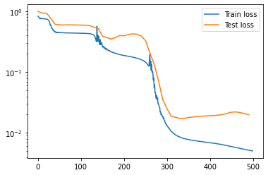
Ok so it’s not nearly as fast as in Jax (maybe 15x slower), but hey you said you wanted PyTorch

import matplotlib.pyplot as plt
plt.plot(np.arange(NUM_EPOCHS),train_losses,label='Train loss')
plt.plot(np.arange(0,NUM_EPOCHS,10),test_losses,label='Test loss')
plt.legend()
plt.yscale('log')

Bonus: Try out model=nn.MLP(trainset.rep_in,trainset.rep_out,group=SO13()).to(device) and see how well it performs on this problem.

Converting Jax functions to PyTorch functions (how it works)

You can use the underlying equivariant bases \(Q\in \mathbb{R}^{n\times r}\) and projection operators \(P = QQ^\top\) in pytorch also.

Since these objects are implicitly defined through LinearOperators, it is not as straightforward as simply calling torch.from_numpy(Q). However, there is a way to use these operators within PyTorch code while preserving any gradients of the operation. We provide the function emlp.reps.pytorch_support.torchify_fn to do this.

import jax
import jax.numpy as jnp
from emlp.reps import V
from emlp.groups import S

For example, let’s setup a representation \(S_4\) consisting of three vectors and one matrix.

W =V(S(4))
rep = 3*W+W**2

First we compute the equivariant basis and equivariant projector linear operators, and then wrap them as functions.

Q = (rep>>rep).equivariant_basis()
P = (rep>>rep).equivariant_projector()

applyQ = lambda v: Q@v
applyP = lambda v: P@v

We can convert any pure pytorch function into a jax function by applying torchify_fn. Now instead of taking jax objects as inputs and outputing jax objects, these functions take in PyTorch objects and output PyTorch objects.

from emlp.nn.pytorch import torchify_fn
applyQ_torch = torchify_fn(applyQ)
applyP_torch = torchify_fn(applyP)

As you would hope, gradients are correctly propagated whether you use the original Jax functions or the torchified pytorch functions.

x_torch = torch.arange(Q.shape[-1]).float().cuda()
x_torch.requires_grad=True
x_jax  = jnp.asarray(x_torch.cpu().data.numpy())

Qx1 = applyQ(x_jax)
Qx2 = applyQ_torch(x_torch)
print("jax output: ",Qx1[:5])
print("torch output: ",Qx2[:5])

jax output:  [0.48484263 0.07053992 0.07053989 0.07053995 1.6988853 ]
torch output:  tensor([0.4848, 0.0705, 0.0705, 0.0705, 1.6989], device='cuda:0',
       grad_fn=<SliceBackward>)

The outputs match, and note that the torch outputs will be on whichever is the default jax device. Similarly, the gradients of the two objects also match:

torch.autograd.grad(Qx2.sum(),x_torch)[0][:5]

tensor([-2.8704,  2.7858, -2.8704,  2.7858, -2.8704], device='cuda:0')

jax.grad(lambda x: (Q@x).sum())(x_jax)[:5]

DeviceArray([-2.8703732,  2.7858496, -2.8703732,  2.7858496, -2.8703732],            dtype=float32)

So you can safely use these torchified functions within your model, and still compute the gradients correctly.

We use this torchify_fn on the projection operators to convert EMLP to pytorch.